CODES / fit / svm (methods)
Methods of the class svm
Contents
eval
Evaluate new samples x
Syntax
- y_hat=svm.eval(x) return the SVM values y_hat of the samples x
- [y_hat,grad]=svm.eval(x) return the gradients grad at x
Example
svm=CODES.fit.svm([1 1;20 2],[1;-1]);
[y_hat,grad]=svm.eval([10 0.5;5 0.6;14 0.8]);
disp([[' y_hat : ';'grad_1 : ';'grad_2 : '] num2str([y_hat';grad'],'%1.3f  ')])
 y_hat :  0.906   1.083   0.509
grad_1 : -0.047  -0.041  -0.055
grad_2 : -0.449  -0.450  -0.814
class
Provides the sign of input y, different than MATLAB sign function for y=0.
Syntax
- lab=svm.class(y) computes labels lab for function values y.
Example
svm=CODES.fit.svm([1;2],[1;-1]);
y=[1;-1;-2;3;0];
lab=svm.class(y);
disp([['   y : ';' lab : ';'sign : '] num2str([y';lab';sign(y')],'%1.3f  ')])
   y : 1.000  -1.000  -2.000   3.000   0.000
 lab : 1.000  -1.000  -1.000   1.000  -1.000
sign : 1.000  -1.000  -1.000   1.000   0.000
See also
eval_classeval_class
Evaluate class of new samples x
Syntax
- lab=svm.eval_class(x) computes the labels lab of the input samples x.
- [lab,y_hat]=svm.eval_class(x) also returns predicted function values y_hat.
Example
svm=CODES.fit.svm([1;2],[1;-1]);
x=[0;1;2;3];
[lab,y_hat]=svm.eval_class(x);
disp([['y_hat : ';'  lab : '] num2str([y_hat';lab'],'%1.3f  ')])
y_hat : 1.198   1.000  -1.000  -1.198
  lab : 1.000   1.000  -1.000  -1.000
See also
classscale
Perform scaling of samples x_unsc
Syntax
- x_sc=svm.scale(x_unsc) scales x_unsc.
Example
svm=CODES.fit.svm([1 1;20 2],[1;-1]);
x_unsc=[1 1;10 1.5;20 2];
x_sc=svm.scale(x_unsc);
disp('        Unscaled             Scaled')
disp([x_unsc x_sc])
        Unscaled             Scaled
    1.0000    1.0000         0         0
   10.0000    1.5000    0.4737    0.5000
   20.0000    2.0000    1.0000    1.0000
See also
unscaleunscale
Perform unscaling of samples x_sc
Syntax
- x_unsc=svm.unscale(x_sc) unscales x_sc.
Example
svm=CODES.fit.svm([1 1;20 2],[1;-1]);
x_sc=[0 0;0.4737 -1;1 1];
x_unsc=svm.unscale(x_sc);
disp('         Scaled             Unscaled')
disp([x_sc x_unsc])
         Scaled             Unscaled
         0         0    1.0000    1.0000
    0.4737   -1.0000   10.0003         0
    1.0000    1.0000   20.0000    2.0000
See also
scaleadd
Retrain svm after adding a new sample (x,y)
Syntax
- svm=svm.add(x,y) adds a new sample x with function value y.
Example
svm=CODES.fit.svm([1;2],[1;-1]);
disp(['Predicted class at x=1.4, ' num2str(svm.eval_class(1.4))])
svm=svm.add(1.5,-1);
disp(['Updated predicted class at x=1.4, ' num2str(svm.eval_class(1.4))])
Predicted class at x=1.4, 1
Updated predicted class at x=1.4, -1
me
Compute the Misclassification Error (ME) for (x,y) (%)
Syntax
- stat=svm.me(x,y) compute the me for (x,y)
- stat=svm.me(x,y,use_balanced) returns Balanced Misclassification Error (BME) if use_balanced is set to true
Description
For a representative (sample,label)  of the domain of interest and predicted labels
  , the classification error is defined as:
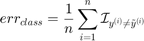
On the other hand, the balanced classification error is defined as:
![$$err_{class}^{bal}=\frac{1}{n}\sum_{i=1}^n\left[w_p\mathcal{I}_{y^{(i)}=+1}\mathcal{I}_{y^{(i)}\neq\tilde{y}^{(i)}}+w_m\mathcal{I}_{y^{(i)}=-1}\mathcal{I}_{y^{(i)}\neq\tilde{y}^{(i)}}\right]$$](svm_method_eq07423943349070457344.png)
where  and
and  are weights computed based on training samples such that:
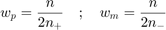
where  is the total number of samples and
  (resp.
  ) is the total number of positive (resp. negative) samples. This weights satisfy a set of condition:
 if all positive or all negative samples are misclassified;
 if all samples are properly classified;
 if all samples are misclassified;
 .
.
This function is typically used to validate meta-models on an independent validation set as in Jiang and Missoum (2014).
Example
f=@(x)x-4;
x=[2;8];y=f(x);
svm=CODES.fit.svm(x,y);
x_t=linspace(0,10,1e4)';y_t=f(x_t);
err=svm.me(x_t,y_t);
bal_err=svm.me(x_t,y_t,true);
disp('On evenly balanced training set, standard and balanced prediction error return same values')
disp([err bal_err])
x=[2;5;8];y=f(x);
svm=CODES.fit.svm(x,y);
err=svm.me(x_t,y_t);
bal_err=svm.me(x_t,y_t,true);
disp('On unevenly balanced training set, standard and balanced prediction error return different values')
disp([err bal_err])
On evenly balanced training set, standard and balanced prediction error return same values
    10    10

On unevenly balanced training set, standard and balanced prediction error return different values
    5.0000    7.5000
See also
auc | mse | rmse | cv | looauc
Returns the Area Under the Curve (AUC) for (x,y) (%)
Syntax
- stat=CODES.fit.svm.auc(x,y) return the AUC stat for the samples (x,y)
- stat=CODES.fit.svm.auc(x,y,ROC) plot the ROC curves if ROC|is set to |true
- [stat,FP,TP]=CODES.fit.svm.auc(...) returns the false positive rate FP and the true positive rate TP
Description
A receiver operating characteristic (ROC) curve Metz (1978) is a graphical representation of the relation between true and false positive predictions for a binary classifier. It uses all possible decision thresholds from the prediction. In the case of SVM classification, thresholds are defined by the SVM values. More specifically, for each threshold a True Positive Rate:
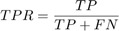
and a False Positive Rate:
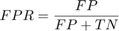
are calculated.  and
and  are the number of true positive and true negative predictions while
  and
and  are the number of false positive and false negative predictions, respectively. The ROC curve represents
  as a function of
  .
.
Once the ROC curve is constructed, the area under the ROC curve (AUC) can be calculated and used as a validation metric. A perfect classifier will have an AUC equal to one. An AUC value of 0.5 indicates no discriminative ability.

Example
f=@(x)x(:,2)-sin(10*x(:,1))/4-0.5;
x=CODES.sampling.cvt(30,2);y=f(x);
svm=CODES.fit.svm(x,y);
auc_val=svm.auc(svm.X,svm.Y);
x_t=rand(1000,2);
y_t=f(x_t);
auc_new=svm.auc(x_t,y_t);
disp(['AUC value over training set : ' num2str(auc_val,'%7.3f')])
disp([' AUC value over testing set : ' num2str(auc_new,'%7.3f')])
AUC value over training set : 100.000
 AUC value over testing set : 95.377
See also
me | mse | rmse | cvN_sv_ratio
Returns the support vector ratio as a percent
Syntax
- stat=svm.N_sv_ratio return the support vector ratio stat
- stat=svm.N_sv_ratio(use_balanced) returns the balanced support vector ratio if use_balanced is set to true
Description
The ratio of support vectors is defined as:

where  is the number of support vectors. On the other hand, the balanced support vector ratio is defined as:
where  and
and  are the number of positive and negative support vectors, respectively. and are weights computed based on training samples such that:
where is the total number of samples and (resp. ) is the total number of positive (resp. negative) samples. This weights satisfy a set of conditions:
 if all positive or all negative samples are support vectors;
 if no samples are support vectors;
 if all samples are support vectors;
 .
.
Example
f=@(x)x-4;
x=[2;8];y=f(x);
svm=CODES.fit.svm(x,y);
Nsv=svm.N_sv_ratio;
bal_Nsv=svm.N_sv_ratio(true);
disp('On an evenly balanced training set, standard and balanced support vector ratios return the same value')
disp([Nsv bal_Nsv])
x=[2;5;8];y=f(x);
svm=CODES.fit.svm(x,y);
Nsv=svm.N_sv_ratio;
bal_Nsv=svm.N_sv_ratio(true);
disp('On an unevenly balanced training set, standard and balanced support vector ratios each return a different value')
disp([Nsv bal_Nsv])
On an evenly balanced training set, standard and balanced support vector ratios return the same value
   100   100

On an unevenly balanced training set, standard and balanced support vector ratios each return a different value
   66.6667   75.0000
See also
loo | cv | chapelle | aucchapelle
Returns Chapelle estimate of the LOO error as a percentage
Syntax
- stat=svm.chapelle returns the Chapelle estimate of the LOO error stat
- stat=svm.chapelle(use_balanced) returns the Chapelle estimate of the balanced LOO error if use_balanced is set to true
Description
This function computes LOO error estimates as derived in Chapelle et al., 2002. Weight used when use_balanced is true are described in loo.
Example
f=@(x)x(:,1)-0.5;
x=CODES.sampling.cvt(30,2);y=f(x);
svm=CODES.fit.svm(x,y);
chap_err=svm.chapelle;
bal_chap_err=svm.chapelle(true);
disp('On an evenly balanced training set, standard and balanced Chapelle errors return the same value')
disp([chap_err bal_chap_err])
x=CODES.sampling.cvt(31,2);y=f(x);
svm=CODES.fit.svm(x,y);
chap_err=svm.chapelle;
bal_chap_err=svm.chapelle(true);
disp('On an unevenly balanced training set, standard and balanced Chapelle errors each return a different value')
disp([chap_err bal_chap_err])
On an evenly balanced training set, standard and balanced Chapelle errors return the same value
   13.3333   13.3333

On an unevenly balanced training set, standard and balanced Chapelle errors each return a different value
   12.9032   12.9167
See also
N_sv_ratio | loo | cv | aucloo
Returns the Leave One Out (LOO) error (%)
Syntax
- stat=svm.loo return the loo error stat
- stat=svm.loo(param,value) use set of parameters param and values value (c.f., parameter table)
Description
Define  the
the  predicted label and
  the predicted label using the SVM trained without the
  sample. The Leave One Out (LOO) error is defined as:
On the other hand, the balanced LOO error is defined as:
![$$err_{loo}^{bal}=\frac{1}{n}\sum_{i=1}^n\left[w_p\mathcal{I}_{l^{(i)}=+1}\mathcal{I}_{\tilde{l}^{(i)}\neq\tilde{l}_{-i}^{(i)}}+w_m\mathcal{I}_{l^{(i)}=-1}\mathcal{I}_{\tilde{l}^{(i)}\neq\tilde{l}_{-i}^{(i)}}\right]$$](svm_method_eq01846700469269783418.png)
and are weights computed based on training samples such that:
where is the total number of samples and (resp. ) is the total number of positive (resp. negative) samples. This weights satisfy a set of condition:
 if all positive or all negative samples are misclassified;
 if no samples are misclassified;
 if all samples are miscalssified;
 .
.
Parameters
| param | value | Description |
|---|---|---|
| 'use_balanced' | logical, {false} | Only for Misclassification Error, uses Balanced Misclassification Error if true> |
| 'metric' | {'me'}, 'mse' | Metric on which LOO procedure is applied, Misclassification Error ('me') or Mean Square Error ('mse') |
Example
f=@(x)x(:,2)-sin(10*x(:,1))/4-0.5;
x=CODES.sampling.cvt(6,2);y=f(x);
svm=CODES.fit.svm(x,y);
loo_err=svm.loo;
bal_loo_err=svm.loo('use_balanced',true);
disp('On evenly balanced training set, standard and balanced loo error return same values')
disp([loo_err bal_loo_err])
x=CODES.sampling.cvt(5,2);y=f(x);
svm=CODES.fit.svm(x,y);
loo_err=svm.loo;
bal_loo_err=svm.loo('use_balanced',true);
disp('On unevenly balanced training set, standard and balanced loo error return different values')
disp([loo_err bal_loo_err])
On evenly balanced training set, standard and balanced loo error return same values
   66.6667   66.6667

On unevenly balanced training set, standard and balanced loo error return different values
   40.0000   41.6667
See also
cv | auc | me | msecv
Returns the Cross Validation (CV) error over 10 folds (%)
Syntax
- stat=svm.cv return the cv error stat
- stat=svm.cv(param,value) use set of parameters param and values value (c.f., parameter table)
Description
This function follow the same outline as the loo but uses a 10 fold CV procedure instead of an fold one. Therefore, the cv and loo are the same for  and cv returns an estimate of loo that is faster to compute for
  .
.
Parameters
| param | value | Description |
|---|---|---|
| 'use_balanced' | logical, {false} | Only for Misclassification Error, uses Balanced Misclassification Error if true> |
| 'metric' | 'auc', {'me'}, 'mse' | Metric on which CV procedure is applied: Area Under the Curve ('auc'), Misclassification Error ('me') or Mean Square Error ('mse') |
Example
f=@(x)x(:,1)-0.5;
x=CODES.sampling.cvt(30,2);y=f(x);
svm=CODES.fit.svm(x,y);
rng(0); % To ensure same CV folds
cv_err=svm.cv;
rng(0);
bal_cv_err=svm.cv('use_balanced',true);
disp('On evenly balanced training set, standard and balanced cv error return same values')
disp([cv_err bal_cv_err])
x=CODES.sampling.cvt(31,2);y=f(x);
svm=CODES.fit.svm(x,y);
rng(0);
cv_err=svm.cv;
rng(0);
bal_cv_err=svm.cv('use_balanced',true);
disp('On unevenly balanced training set, standard and balanced cv error return different values')
disp([cv_err bal_cv_err])
On evenly balanced training set, standard and balanced cv error return same values
    6.6667    6.6667

On unevenly balanced training set, standard and balanced cv error return different values
    6.6667    6.6736
See also
loo | auc | me | mseclass_change
Compute the change of class between two meta-models over a sample x (%)
Syntax
- stat=svm.class_change(svm_old,x) compute the change of class of the sample x from meta-model svm_old to meta-model svm
Description
This metric was used in Basudhar and Missoum (2008) as convergence metric and is defined as:
where  is the number of convergence samples and
  (resp.
  ) is the convergence predicted label using svm_old (resp. svm).
Example
f=@(x)x-4;
x=[2;8];y=f(x);
svm=CODES.fit.svm(x,y);
x_t=linspace(0,10,1e4)';y_t=f(x_t);
err=svm.me(x_t,y_t);
svm_new=svm.add(5,f(5));
err_new=svm_new.me(x_t,y_t);
class_change=svm_new.class_change(svm,x_t);
disp(['Absolute change in prediction error : ' num2str(abs(err_new-err))])
disp(['Class change : ' num2str(class_change)])
Absolute change in prediction error : 5
Class change : 15
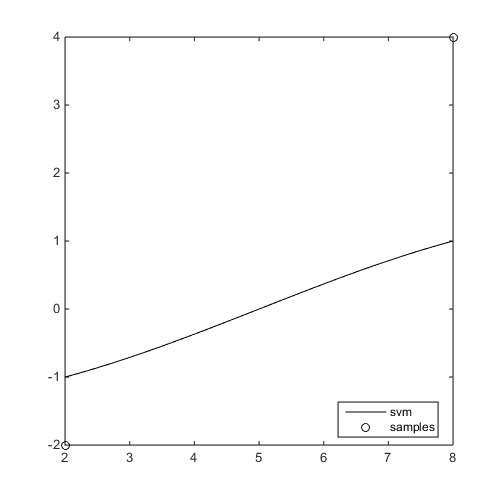
plot
Display the meta-model svm
Syntax
- svm.plot plot the meta-model svm
- svm.plot(param,value) use set of parameters param and values value (c.f., parameter table)
- h=svm.plot(...) returns graphical handles
Parameters
| param | value | Description |
|---|---|---|
| 'new_fig' | logical, {false} | Create a new figure |
| 'lb' | numeric, {svm.lb_x} | Lower bound of plot |
| 'ub' | numeric, {svm.ub_x} | Upper bound of plot |
| 'samples' | logical, {true} | Plot training samples |
| 'lsty' | string, {'k-'} | Line style (1D), see also LineSpec |
| 'psty' | string, {'ko'} | Samples style, see also LineSpec |
| 'legend' | logical, {true} | Add legend |
Example
f=@(x)x-4;
x=[2;8];y=f(x);
svm=CODES.fit.svm(x,y);
svm.plot('new_fig',true)
See also
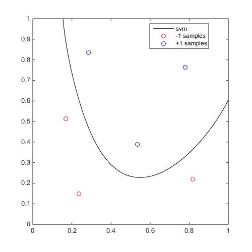
isoplotisoplot
Display the 0 isocontour of the SVM svm
Syntax
- svm.isoplot plots the 0 isocontour of the meta-model svm
- svm.isoplot(param,value) uses set of parameters param and values value (see parameter table)
- h=svm.isoplot(...) returns graphical handles
Parameters
| param | value | Description |
|---|---|---|
| 'new_fig' | logical, {false} | Create a new figure. |
| 'th' | numeric, {0} | Isovalue to plot. |
| 'lb' | numeric, {svm.lb_x} | Lower bound of plot. |
| 'ub' | numeric, {svm.ub_x} | Upper bound of plot. |
| 'samples' | logical, {true} | Plot training samples. |
| 'mlsty' | string, {'r-'} | Line style for -1 domain (1D), see also LineSpec. |
| 'plsty' | string, {'b-'} | Line style for +1 domain (1D), see also LineSpec. |
| 'bcol' | string, {'k'} | Boundary color, see also LineSpec. |
| 'mpsty' | string, {'ro'} | -1 samples style, see also LineSpec. |
| 'ppsty' | string, {'bo'} | +1 samples style, see also LineSpec. |
| 'use_light' | logical, {true} | Use light (3D). |
| 'prev_leg' | cell, { {} } | Previous legend entry. |
| 'legend' | logical, {true} | Add legend. |
| 'sv' | logical, {true} | Plot support vectors |
| 'msvsty' | string, {'r+'} | -1 samples style |
| 'psvsty' | string, {'b+'} | +1 samples style |
Example
f=@(x)x(:,2)-sin(10*x(:,1))/4-0.5;
x=CODES.sampling.cvt(6,2);y=f(x);
svm=CODES.fit.svm(x,y);
svm.isoplot('new_fig',true,'lb',[0 0],'ub',[1 1],'sv',false)
point_dist
Returns the minimum, maximum, and mean values of the pairwise distances between +1 and -1 training samples of svm in the scaled domain. The mean value is used for 'param_select' set to 'fast' and as initial guess for other selection strategies.
Syntax
- [lb,ub,mean_dist]=svm.point_dist
Example
f=@(x)x(:,1)-0.5;
X=CODES.sampling.cvt(20,2);Y=f(X);
svm=CODES.fit.svm(X,Y,'param_select','fast');
[lb,ub,mean_dist]=svm.point_dist;
disp(['SVM theta value : ' num2str(svm.theta,'%1.3f  ')])
disp(['  Mean distance : ' num2str(mean_dist,'%1.3f  ')])
SVM theta value : 0.768
  Mean distance : 0.768
References
- Basudhar et al. (2008): Basudhar A., Missoum S., (2008) Adaptive explicit decision functions for probabilistic design and optimization using support vector machines. Computers & Structures 86(19):1904-1917 - DOI
- Chapelle et al. (2002): Chapelle, O., Vapnik, V., Bousquet, O., & Mukherjee, S., (2002) Choosing multiple parameters for support vector machines. Machine Learning 46(1-3):131-159 - DOI
- Jiang et al. (2014): Jiang P., Missoum S., (2014) Optimal SVM parameter selection for non-separable and unbalanced datasets. Structural and Multidisciplinary Optimization 50(4):523-535 - DOI
- Metz (1978): Metz C. E., (2008) Basic principles of ROC analysis. Seminars in nuclear medicine 8(4):283-298 - DOI
Copyright © 2015 Computational Optimal Design of Engineering Systems (CODES) Laboratory. University of Arizona.
|
|
Computational Optimal Design of Engineering Systems |

|