kriging

This file is a complete demo of the capability of the kriging class from the CODES toolbox.

Documentation
Set rng
Simple example
Simple example for regression
Compare CODES and DACE implementation
References

Documentation

The documentation for the kriging class can be found here.

Set rng

Set random number generator seed:

rng(1)

Simple example

Define a simple sinusoidal problem:

f=@(x)x.*sin(x);
x=CODES.sampling.cvt(10,1,'lb',0,'ub',10);
y=f(x);

Build and plot a Kriging without CI:

kr=CODES.fit.kriging(x,y);

figure('Position',[200 200 500 500])
plot(linspace(0,10,100)',f(linspace(0,10,100)'),'ro--')
hold on
kr.plot('prev_leg',{'true'},'psty','k^','lb',0,'ub',10,'CI',false)

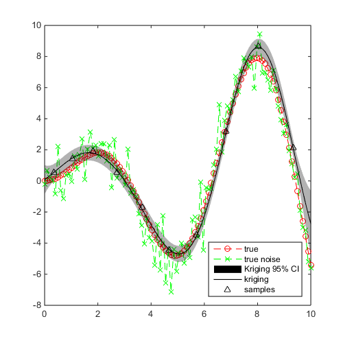
Simple example for regression

Define a simple sinusoidal problem with noise:

f=@(x)x.*sin(x);
f_noise=@(x)x.*sin(x)+normrnd(0,1,size(x,1),1);
x=CODES.sampling.cvt(10,1,'lb',0,'ub',10);
y=f_noise(x);

Build and plot a Kriging:

kr=CODES.fit.kriging(x,y,'regression',true);

figure('Position',[200 200 500 500])
plot(linspace(0,10,100)',f(linspace(0,10,100)'),'ro--')
hold on
plot(linspace(0,10,100)',f_noise(linspace(0,10,100)'),'gx--')
kr.plot('prev_leg',{'true','true noise'},'psty','k^','lb',0,'ub',10)

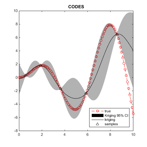
Compare CODES and DACE implementation

Define a simple sinusoidal problem:

f=@(x)x.*sin(x);
x=CODES.sampling.cvt(5,1,'lb',0,'ub',10);
y=f(x);

Build and plot both Kriging:

kr=CODES.fit.kriging(x,y);
kr_dace=CODES.fit.kriging(x,y,'solver','DACE','theta',1,...
    'theta_min',0.01,'theta_max',100);

figure('Position',[200 200 500 500])
plot(linspace(0,10,100)',f(linspace(0,10,100)'),'ro--')
hold on
kr.plot('prev_leg',{'true'},'psty','k^','lb',0,'ub',10)
title('CODES')

figure('Position',[200 200 500 500])
plot(linspace(0,10,100)',f(linspace(0,10,100)'),'ro--')
hold on
kr_dace.plot('prev_leg',{'true'},'psty','k^','lb',0,'ub',10)
title('DACE')

Compare gradients

x_t=unifrnd(0,10,5,1);
[CODES_mean,CODES_var,CODES_mean_gr,CODES_var_gr]=kr.eval_all(x_t);
[DACE_mean,DACE_var,DACE_mean_gr,DACE_var_gr]=kr_dace.eval_all(x_t);

fprintf('\n%15s | %17s | %17s | %17s\n','Mean','Variance','Mean grad','Var grad');
disp(num2str([CODES_mean DACE_mean CODES_var DACE_var CODES_mean_gr DACE_mean_gr CODES_var_gr DACE_var_gr],'%8.3f %8.3f | %8.3f %8.3f | %8.3f %8.3f | %8.3f %8.3f'));

           Mean |          Variance |         Mean grad |          Var grad
-1.192   -1.189 |    1.196    1.193 |    3.164    3.168 |    4.703    4.694
 1.340    1.340 |    0.314    0.319 |    1.399    1.399 |   -0.115   -0.124
-3.087   -3.092 |    2.410    2.396 |   -0.421   -0.422 |    0.768    0.767
 4.435    4.443 |    7.405    8.074 |   -2.717   -2.713 |    6.427    7.793
 5.440    5.446 |    4.636    4.886 |   -2.433   -2.427 |    7.715    8.516

References

DACE Toolbox

Computational Optimal Design of
Engineering Systems

References

Copyright © 2015 Computational Optimal Design of Engineering Systems (CODES) Laboratory. University of Arizona.