Examples / Adaptive sampling / anti_lock

This file is a complete demo of the capability of the anti_lock function from the CODES toolbox.

Contents

Documentation

The documentation for the anti-lock function can be found here.

Set rng

Set random number generator seed:

rng(0)

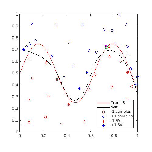
Simple example

Define a simple sinusoidal problem:

f=@(x)x(:,2)-sin(10*x(:,1))/4-0.5;
x=CODES.sampling.cvt(30,2);
y=f(x);

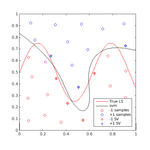
Train an SVM, find a "max-min" sample and plot it:

svm=CODES.fit.svm(x,y);
x_al=CODES.sampling.anti_lock(svm,[0 0],[1 1]);

[X,Y]=meshgrid(linspace(0,1,100));
Z=reshape(f([X(:) Y(:)]),100,100);

figure('Position',[200 200 500 500])
contour(X,Y,Z,[0 0],'r')
hold on
svm.isoplot('lb',[0 0],'ub',[1 1],'prev_leg',{'True LS'})
plot(x_al(1),x_al(2),'ms')
axis square

Parallel vs serial and MultiStart

Start a parallel pool:

gcp;

Compare compuational time of different scenarios to compute 10 "anti-locking" samples:

CODES.common.disp_box('Using Matlab MultiStart')
tic;
svm=CODES.fit.svm(x,y);
CODES.sampling.anti_lock(svm,[0 0],[1 1],'nb',10,'MultiStart','MATLAB');
disp(['Serial : ' CODES.common.time(toc)])
tic;
svm=CODES.fit.svm(x,y,'UseParallel',true);
CODES.sampling.anti_lock(svm,[0 0],[1 1],'nb',10,'MultiStart','MATLAB');
disp(['Parallel : ' CODES.common.time(toc)])
CODES.common.disp_box('Using CODES MultiStart')
tic;
svm=CODES.fit.svm(x,y);
CODES.sampling.anti_lock(svm,[0 0],[1 1],'nb',10,'MultiStart','CODES');
disp(['Serial : ' CODES.common.time(toc)])
tic;
svm=CODES.fit.svm(x,y,'UseParallel',true);
CODES.sampling.anti_lock(svm,[0 0],[1 1],'nb',10,'MultiStart','CODES');
disp(['Parallel : ' CODES.common.time(toc)])

 
###########################
# Using Matlab MultiStart #
###########################
 
Serial : 44s
Parallel : 29s
 
##########################
# Using CODES MultiStart #
##########################
 
Serial : 35s
Parallel : 22s

Display intermediate steps

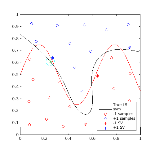
Display intermediate elements of the "anti-locking" calculation:

rng(0);
f=@(x)x(:,2)-sin(10*x(:,1))/4-0.5;
x=CODES.sampling.cvt(30,2);
y=f(x);

svm=CODES.fit.svm(x,y,'UseParallel',true);
[x_al,adds]=CODES.sampling.anti_lock(svm,[0 0],[1 1]);

[X,Y]=meshgrid(linspace(0,1,100));
Z=reshape(f([X(:) Y(:)]),100,100);

figure('Position',[200 200 500 500])
contour(X,Y,Z,[0 0],'r')
hold on
svm.isoplot('lb',[0 0],'ub',[1 1],'prev_leg',{'True LS'})
plot(adds{1}(1),adds{1}(2),'go')        % Plot center x_c
plot(adds{2}(:,1),adds{2}(:,2),'c--')   % Plot region boundary ||x-x_c||-R<=0
plot(x_al(1),x_al(2),'ms')
axis square

Parallel update

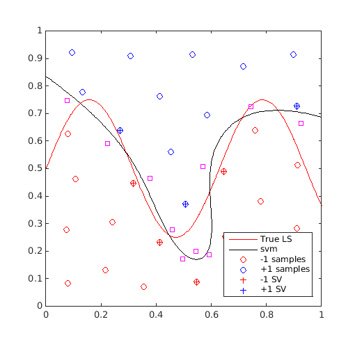
On the same example, find 10 max-min samples and plot them:

f=@(x)x(:,2)-sin(10*x(:,1))/4-0.5;
x=CODES.sampling.cvt(30,2);
y=f(x);

svm=CODES.fit.svm(x,y,'UseParallel',true);
x_al=CODES.sampling.anti_lock(svm,[0 0],[1 1],'nb',10);

[X,Y]=meshgrid(linspace(0,1,100));
Z=reshape(f([X(:) Y(:)]),100,100);

figure('Position',[200 200 500 500])
contour(X,Y,Z,[0 0],'r')
hold on
svm.isoplot('lb',[0 0],'ub',[1 1],'prev_leg',{'True LS'})
plot(x_al(:,1),x_al(:,2),'ms')
axis square

Sequential refinement

On the same example, for 20 iterations, find a "anti-locking" sample and update the svm with that sample:

f=@(x)x(:,2)-sin(10*x(:,1))/4-0.5;
x=CODES.sampling.cvt(30,2);
y=f(x);

svm=CODES.fit.svm(x,y,'UseParallel',true);

[X,Y]=meshgrid(linspace(0,1,100));
Z=reshape(f([X(:) Y(:)]),100,100);

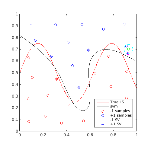
Plot the first and last iterations:

[x_al,adds]=CODES.sampling.anti_lock(svm,[0 0],[1 1]);
svm=svm.add(x_al,f(x_al));

figure('Position',[200 200 500 500])
contour(X,Y,Z,[0 0],'r')
hold on
svm.isoplot('lb',[0 0],'ub',[1 1],'prev_leg',{'True LS'})
plot(adds{1}(1),adds{1}(2),'go')        % Plot center x_c
plot(adds{2}(:,1),adds{2}(:,2),'c--')   % Plot region boundary ||x-x_c||-R<=0
plot(x_al(:,1),x_al(:,2),'ms')
axis square

for i=2:20
    [x_al,adds]=CODES.sampling.anti_lock(svm,[0 0],[1 1]);
    svm=svm.add(x_al,f(x_al));
end

figure('Position',[200 200 500 500])
contour(X,Y,Z,[0 0],'r')
hold on
svm.isoplot('lb',[0 0],'ub',[1 1],'prev_leg',{'True LS'})
plot(adds{1}(1),adds{1}(2),'go')        % Plot center x_c
plot(adds{2}(:,1),adds{2}(:,2),'c--')   % Plot region boundary ||x-x_c||-R<=0
plot(x_al(:,1),x_al(:,2),'ms')
axis square

A video of this sequential update can be found here.

Copyright © 2015 Computational Optimal Design of Engineering Systems (CODES) Laboratory. University of Arizona.

Computational Optimal Design of Engineering Systems

Published with MATLAB® R2014b