Examples / Adaptive sampling / cvt

This file is a complete demo of the capability of the cvt function from the CODES toolbox.

Documentation
Set rng
Simple example
Restricted DOE
Distribution tailored DOE

Documentation

The documentation for the cvt function can be found here.

Set rng

Set random number generator seed:

rng(0)

Simple example

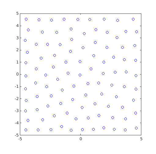
Build a simple CVT DOE within a square of side length 10 centered on the origin:

DOE=CODES.sampling.cvt(100,2,'lb',[-5 -5],'ub',[5 5]);

figure('Position',[200 200 500 500])
plot(DOE(:,1),DOE(:,2),'bo')
axis square
axis([-5 5 -5 5])

Restricted DOE

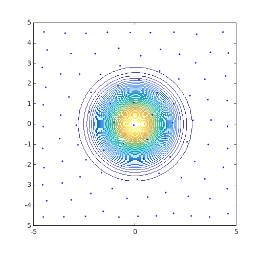
Observe the previous DOE overlayed with a normal distribution:

JPDF=@(x)mvnpdf(x,[0 0],[1 0;0 1]);
[X,Y]=meshgrid(linspace(-5,5,100));
Z=reshape(JPDF([X(:) Y(:)]),100,100);

figure('Position',[200 200 500 500])
contour(X,Y,Z,50)
hold on
plot(DOE(:,1),DOE(:,2),'b.')
axis square
axis([-5 5 -5 5])

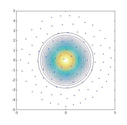
A better DOE would be to have CVT samples restricted within a circle:

DOE=CODES.sampling.cvt(100,2,'lb',[-5 -5],'ub',[5 5],'region',@(x)5-pdist2(x,[0 0]));

figure('Position',[200 200 500 500])
contour(X,Y,Z,50)
hold on
plot(DOE(:,1),DOE(:,2),'b.')
axis square
axis([-5 5 -5 5])

Sum of square change at iteration 1: 4.837e-03
Sum of square change at iteration 2: 2.711e-03
Sum of square change at iteration 3: 1.701e-03; Predicted relative change : 2.260e-01
Sum of square change at iteration 4: 9.493e-04; Predicted relative change : 2.083e-01
Sum of square change at iteration 5: 6.000e-04; Predicted relative change : 1.363e-01
Sum of square change at iteration 6: 3.923e-04; Predicted relative change : 8.108e-02
Sum of square change at iteration 7: 2.986e-04; Predicted relative change : 1.211e-25
Sum of square change at iteration 8: 2.412e-04; Predicted relative change : 6.006e-14
Sum of square change at iteration 9: 1.981e-04; Predicted relative change : 3.152e-58

Distribution tailored DOE

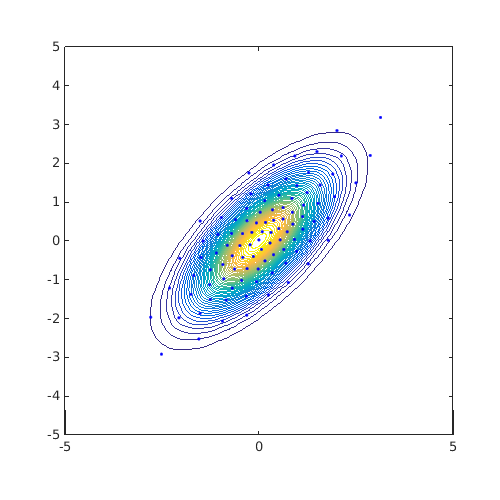
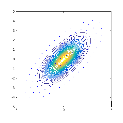
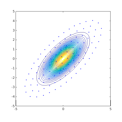
The previous example relied on previous knowledge for the definition of the region. Another idea is to use isovalues of the target distribution as the region boundary. For example, consider a correlated Gaussian example as follows:

JPDF=@(x)mvnpdf(x,[0 0],[1 0.7;0.7 1]);
ndummies=mvnrnd([0 0],[1 0.7;0.7 1],1e5);
[X,Y]=meshgrid(linspace(-5,5,100));
Z=reshape(JPDF([X(:) Y(:)]),100,100);

tic;
DOE=CODES.sampling.cvt(100,2,'lb',[-5 -5],'ub',[5 5],...
    'dummies',ndummies,'display',false);
disp(['Time to find CVT with prescribed dummies : ' CODES.common.time(toc)])
tic;
DOE1=CODES.sampling.cvt(100,2,'lb',[-5 -5],'ub',[5 5],...
    'dummies',ndummies,'kmeans',true);
disp(['Time to find CVT with prescribed dummies and matlab built-in kmeans : ' CODES.common.time(toc)])
tic;
DOE2=CODES.sampling.cvt(100,2,'lb',[-5 -5],'ub',[5 5],...
    'region',@(x)JPDF(x)-JPDF([4 4]),'display',false);
disp(['Time to find CVT with shuffled Halton dummies : ' CODES.common.time(toc)])
tic;
DOE3=CODES.sampling.cvt(100,2,'lb',[-5 -5],'ub',[5 5],...
    'region',@(x)JPDF(x)-JPDF([4 4]),'kmeans',true);
disp(['Time to find CVT with matlab built-in kmeans : ' CODES.common.time(toc)])

figure('Position',[200 200 500 500])
contour(X,Y,Z,50)
hold on
plot(DOE(:,1),DOE(:,2),'b.')
axis square
axis([-5 5 -5 5])

figure('Position',[200 200 500 500])
contour(X,Y,Z,50)
hold on
plot(DOE1(:,1),DOE1(:,2),'b.')
axis square
axis([-5 5 -5 5])

figure('Position',[200 200 500 500])
contour(X,Y,Z,50)
hold on
plot(DOE2(:,1),DOE2(:,2),'b.')
axis square
axis([-5 5 -5 5])

figure('Position',[200 200 500 500])
contour(X,Y,Z,50)
hold on
plot(DOE3(:,1),DOE3(:,2),'b.')
axis square
axis([-5 5 -5 5])

Time to find CVT with prescribed dummies : 4s
Warning: Failed to converge in 100 iterations. 
Time to find CVT with prescribed dummies and matlab built-in kmeans : 11s
Time to find CVT with shuffled Halton dummies : 5s
Warning: Failed to converge in 100 iterations. 
Time to find CVT with matlab built-in kmeans : 12s