Examples / Adaptive sampling / gmm

This file is a complete demo of the capability of the gmm function from the CODES toolbox.

Documentation
Set rng
Simple example
Comparison of Computational Time for: Parallel and Serial; With and Without Derivative; and Matlab and CODES Multistart:
Parallel update
Sequential refinement

Documentation

The documentation for the gmm function can be found here.

Set rng

Set random number generator seed:

rng(0)

Simple example

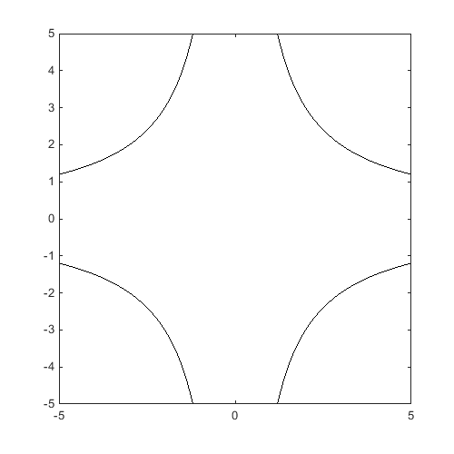
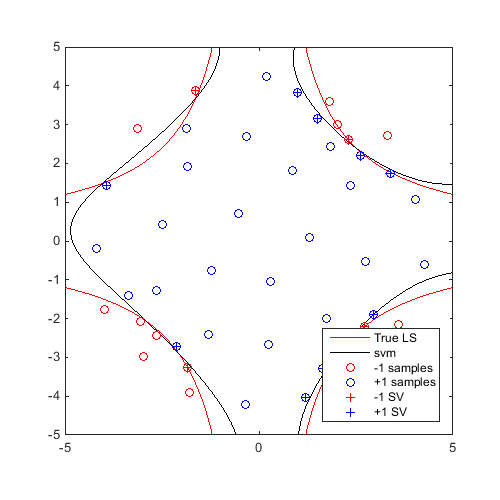
Define a 2D reliability problem with 4 failure domains:

f=@CODES.test.inverse_2D;
[X,Y]=meshgrid(linspace(-5,5,100));
Z=reshape(f([X(:) Y(:)]),100,100);
figure('Position',[200 200 500 500])
contour(X,Y,Z,[0 0],'k')

Obtain a DOE:

x=CODES.sampling.cvt(30,2,'lb',[-5 -5],'ub',[5 5],'region',@(x)5-pdist2(x,[0 0]));
y=f(x);

Sum of square change at iteration 1: 3.572e-03
Sum of square change at iteration 2: 1.587e-03
Sum of square change at iteration 3: 8.792e-04; Predicted relative change : 2.528e-01
Sum of square change at iteration 4: 5.334e-04; Predicted relative change : 2.163e-01
Sum of square change at iteration 5: 3.657e-04; Predicted relative change : 1.472e-01
Sum of square change at iteration 6: 2.899e-04; Predicted relative change : 6.599e-02
Sum of square change at iteration 7: 2.295e-04; Predicted relative change : 5.380e-02
Sum of square change at iteration 8: 2.055e-04; Predicted relative change : 2.675e-02
Sum of square change at iteration 9: 1.756e-04; Predicted relative change : 1.477e-02
Sum of square change at iteration 10: 1.511e-04; Predicted relative change : 2.727e-03
Sum of square change at iteration 11: 1.251e-04; Predicted relative change : 1.180e-03
Sum of square change at iteration 12: 1.091e-04; Predicted relative change : 5.083e-04
Sum of square change at iteration 13: 9.756e-05; Predicted relative change : 2.180e-04

Derive and check log JPDF and gradient (normal distribution):

logjpdf=@(x)sum(-0.5*x.^2-0.5*log(2*pi),2);     % equivalent to logjpdf=@(x)sum(log(normpdf(x)),2);
dlogjpdf=@(x)-x;
test_rng=@(N)normrnd(0,1,[N 2]);                % normal random sampler for optimization starting points

x_grad=[0.1 0.1;0.3 0.5;0.8 0.3;0.5 0.5];
grad=dlogjpdf(x_grad);
grad_fd=CODES.common.grad_fd(logjpdf,x_grad);

disp([['Analytical gradients :';...
       '                      ';...
       '  Finite differences :';...
       '                      '] num2str([grad';grad_fd'],'%1.3f  ')])

Analytical gradients :-0.100  -0.300  -0.800  -0.500
                      -0.100  -0.500  -0.300  -0.500
  Finite differences :-0.100  -0.300  -0.800  -0.500
                      -0.100  -0.500  -0.300  -0.500

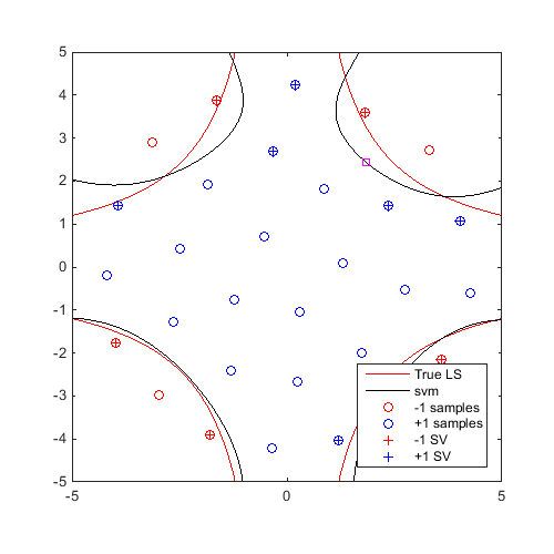
Train an SVM, then find and plot a generalized "max-min" sample:

svm=CODES.fit.svm(x,y);
x_gmm=CODES.sampling.gmm(svm,logjpdf,test_rng,'dlogjpdf',dlogjpdf);

figure('Position',[200 200 500 500])
contour(X,Y,Z,[0 0],'r')
hold on
svm.isoplot('lb',[-5 -5],'ub',[5 5],'prev_leg',{'True LS'})
plot(x_gmm(1),x_gmm(2),'ms')
axis square

Comparison of Computational Time for: Parallel and Serial; With and Without Derivative; and Matlab and CODES Multistart:

Start a parallel pool:

gcp;

Compare compuational time of different scenarios to compute 10 generalized "max-min" samples

CODES.common.disp_box('Using Matlab MultiStart')
tic;
svm=CODES.fit.svm(x,y);
CODES.sampling.gmm(svm,logjpdf,test_rng,'nb',10,'MultiStart','MATLAB');
disp(['Serial without derivative : ' CODES.common.time(toc)])
tic;
svm=CODES.fit.svm(x,y,'UseParallel',true);
CODES.sampling.gmm(svm,logjpdf,test_rng,'nb',10,'MultiStart','MATLAB');
disp(['Parallel without derivative: ' CODES.common.time(toc)])
tic;
svm=CODES.fit.svm(x,y);
CODES.sampling.gmm(svm,logjpdf,test_rng,'dlogjpdf',dlogjpdf,'nb',10,'MultiStart','MATLAB');
disp(['Serial with derivative: ' CODES.common.time(toc)])
tic;
svm=CODES.fit.svm(x,y,'UseParallel',true);
CODES.sampling.gmm(svm,logjpdf,test_rng,'dlogjpdf',dlogjpdf,'nb',10,'MultiStart','MATLAB');
disp(['Parallel with derivative: ' CODES.common.time(toc)])
CODES.common.disp_box('Using CODES MultiStart')
tic;
svm=CODES.fit.svm(x,y);
CODES.sampling.gmm(svm,logjpdf,test_rng,'nb',10,'MultiStart','CODES');
disp(['Serial without derivative : ' CODES.common.time(toc)])
tic;
svm=CODES.fit.svm(x,y,'UseParallel',true);
CODES.sampling.gmm(svm,logjpdf,test_rng,'nb',10,'MultiStart','CODES');
disp(['Parallel without derivative: ' CODES.common.time(toc)])
tic;
svm=CODES.fit.svm(x,y);
CODES.sampling.gmm(svm,logjpdf,test_rng,'dlogjpdf',dlogjpdf,'nb',10,'MultiStart','CODES');
disp(['Serial with derivative: ' CODES.common.time(toc)])
tic;
svm=CODES.fit.svm(x,y,'UseParallel',true);
CODES.sampling.gmm(svm,logjpdf,test_rng,'dlogjpdf',dlogjpdf,'nb',10,'MultiStart','CODES');
disp(['Parallel with derivative: ' CODES.common.time(toc)])

 
###########################
# Using Matlab MultiStart #
###########################
 
Serial without derivative : 23s
Parallel without derivative: 14s
Serial with derivative: 26s
Parallel with derivative: 15s
 
##########################
# Using CODES MultiStart #
##########################
 
Serial without derivative : 23s
Parallel without derivative: 12s
Serial with derivative: 25s
Parallel with derivative: 12s

Parallel update

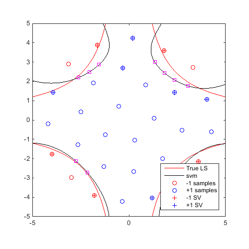
On the same example, find and plot 10 generalized "max-min" samples:

f=@CODES.test.inverse_2D;
x=CODES.sampling.cvt(30,2,'lb',[-5 -5],'ub',[5 5],'region',@(x)5-pdist2(x,[0 0]));
y=f(x);

svm=CODES.fit.svm(x,y,'UseParallel',true);
x_gmm=CODES.sampling.gmm(svm,logjpdf,test_rng,'dlogjpdf',dlogjpdf,'nb',10);

[X,Y]=meshgrid(linspace(-5,5,100));
Z=reshape(f([X(:) Y(:)]),100,100);

figure('Position',[200 200 500 500])
contour(X,Y,Z,[0 0],'r')
hold on
svm.isoplot('lb',[-5 -5],'ub',[5 5],'prev_leg',{'True LS'})
plot(x_gmm(:,1),x_gmm(:,2),'ms')
axis square

Sum of square change at iteration 1: 3.572e-03
Sum of square change at iteration 2: 1.587e-03
Sum of square change at iteration 3: 8.792e-04; Predicted relative change : 2.528e-01
Sum of square change at iteration 4: 5.334e-04; Predicted relative change : 2.163e-01
Sum of square change at iteration 5: 3.657e-04; Predicted relative change : 1.472e-01
Sum of square change at iteration 6: 2.899e-04; Predicted relative change : 6.599e-02
Sum of square change at iteration 7: 2.295e-04; Predicted relative change : 5.380e-02
Sum of square change at iteration 8: 2.055e-04; Predicted relative change : 2.675e-02
Sum of square change at iteration 9: 1.756e-04; Predicted relative change : 1.477e-02
Sum of square change at iteration 10: 1.511e-04; Predicted relative change : 2.727e-03
Sum of square change at iteration 11: 1.251e-04; Predicted relative change : 1.180e-03
Sum of square change at iteration 12: 1.091e-04; Predicted relative change : 5.083e-04
Sum of square change at iteration 13: 9.756e-05; Predicted relative change : 2.180e-04

Sequential refinement

On the same example, for 20 iterations, find a "max-min" sample and update the svm:

f=@CODES.test.inverse_2D;
x=CODES.sampling.cvt(30,2,'lb',[-5 -5],'ub',[5 5],'region',@(x)5-pdist2(x,[0 0]));
y=f(x);

svm=CODES.fit.svm(x,y,'UseParallel',true);

[X,Y]=meshgrid(linspace(-5,5,100));
Z=reshape(f([X(:) Y(:)]),100,100);

Sum of square change at iteration 1: 3.572e-03
Sum of square change at iteration 2: 1.587e-03
Sum of square change at iteration 3: 8.792e-04; Predicted relative change : 2.528e-01
Sum of square change at iteration 4: 5.334e-04; Predicted relative change : 2.163e-01
Sum of square change at iteration 5: 3.657e-04; Predicted relative change : 1.472e-01
Sum of square change at iteration 6: 2.899e-04; Predicted relative change : 6.599e-02
Sum of square change at iteration 7: 2.295e-04; Predicted relative change : 5.380e-02
Sum of square change at iteration 8: 2.055e-04; Predicted relative change : 2.675e-02
Sum of square change at iteration 9: 1.756e-04; Predicted relative change : 1.477e-02
Sum of square change at iteration 10: 1.511e-04; Predicted relative change : 2.727e-03
Sum of square change at iteration 11: 1.251e-04; Predicted relative change : 1.180e-03
Sum of square change at iteration 12: 1.091e-04; Predicted relative change : 5.083e-04
Sum of square change at iteration 13: 9.756e-05; Predicted relative change : 2.180e-04

Plot first and last iteration:

x_gmm=CODES.sampling.gmm(svm,logjpdf,test_rng,'dlogjpdf',dlogjpdf);
svm=svm.add(x_gmm,f(x_gmm));

figure('Position',[200 200 500 500])
contour(X,Y,Z,[0 0],'r')
hold on
svm.isoplot('lb',[-5 -5],'ub',[5 5],'prev_leg',{'True LS'})
plot(x_gmm(:,1),x_gmm(:,2),'ms')
axis square
axis square

for i=2:20
    x_gmm=CODES.sampling.gmm(svm,logjpdf,test_rng,'dlogjpdf',dlogjpdf);
    svm=svm.add(x_gmm,f(x_gmm));
end

figure('Position',[200 200 500 500])
contour(X,Y,Z,[0 0],'r')
hold on
svm.isoplot('lb',[-5 -5],'ub',[5 5],'prev_leg',{'True LS'})
plot(x_gmm(:,1),x_gmm(:,2),'ms')
axis square
axis square

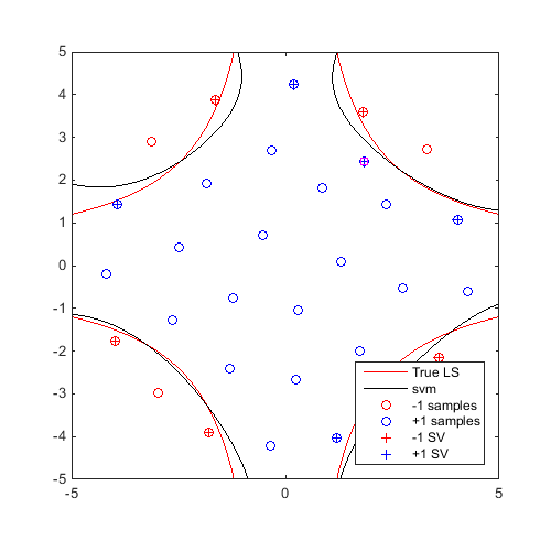
A video of this sequential update can be found here.

Computational Optimal Design of
Engineering Systems