CODES / sampling / gmm

Find a generalized "max-min" sample

Syntax
Description
Parameters
Example
Mini Tutorial
References
See also

Syntax

x_gmm=CODES.sampling.gmm(M,logjpdf,rng) finds a generalized "max-min" sample x_gmm such that M.eval(x)=0, for the log joint probability density function logjpdf. rng is a sampler or a set of points used to determine starting points for the optimization.
x_gmm=CODES.sampling.gmm(...,param,value) uses a list of parameters param and values value (see, parameter table).

Description

This function finds a generalized "max-min" sample as introduced in Lacaze and Missoum (2014):

$\begin{array}{rl}x_{mm}=\mathop{\arg\max}\limits_{x}&\mathbf{f}_X(x)^{\frac{1}{d}}\mathop{\min}\limits_{i}\left|\left|x-x^{(i)}\right|\right|\\\textbf{s.t.} & s(x)=0\\&l_j\leq x_j\leq u_j\end{array}$

where $x^{(.)}$ are the existing samples used to train $s$ , a meta-model (an SVM in Lacaze's work) and $\mathbf{f}_X$ is the probability density function of $X$ . The numerical implementation of this optimization problem follows the steps highlighted in Lacaze and Missoum (2014) regarding the use of the Chebychev distance (infinite norm). This problem being made differentiable, it is then solved using multi-start SQP.

Note that the joint PDF $\mathbf{f}_{\mathbf{X}}$ can be as general as desired including a mix of marginals, dependence structures and copulas.

Parameters

param value Description

'dlogjpdf' function_handle, { [ ] } Gradient of the log of the joint pdf. Must return an (M.dim x n_t) matrix where n_t is the number of samples passed to the function.

'nb' positive integer, {1} Number of "max-min" samples requested ( 'nb' ≥ 2 is refered to as parallel, see Lacaze and Missoum (2014))

'intensity' positive integer, {30} Number of starting points for the multi-start SQP algorithm

'UseParallel' logical, {M.UseParallel} Should parallel set up be used

'MultiStart' {'CODES'}, 'MATLAB' Defines whether MATLAB or CODES multistart fmincon should be used.

'Display' {'off'}, 'iter', 'final' Defines the verbose level.

'sign' {'both'}, 'plus', 'minus' Search generalized "max-min" using all samples, only +1 samples or -1 samples

`param`	`value`	Description
'dlogjpdf'	`function_handle`, { [ ] }	Gradient of the log of the joint pdf. Must return an `(M.dim x n_t)` matrix where `n_t` is the number of samples passed to the function.
'nb'	positive integer, {1}	Number of "max-min" samples requested ( 'nb' ≥ 2 is refered to as parallel, see Lacaze and Missoum (2014))
'intensity'	positive integer, {30}	Number of starting points for the multi-start SQP algorithm
'UseParallel'	logical, {`M.UseParallel`}	Should parallel set up be used
'MultiStart'	{'CODES'}, 'MATLAB'	Defines whether MATLAB or CODES multistart fmincon should be used.
'Display'	{'off'}, 'iter', 'final'	Defines the verbose level.
'sign'	{'both'}, 'plus', 'minus'	Search generalized "max-min" using all samples, only +1 samples or -1 samples

In addition, options from MultiStart can be used as well, when 'MultiStart' is set to 'MATLAB'.

Example

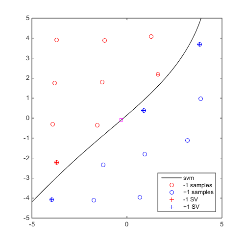
Compute and plot a generalized "max-min" sample

DOE=CODES.sampling.cvt(20,2,'lb',[-5 -5],'ub',[5 5]);
svm=CODES.fit.svm(DOE,DOE(:,1)-DOE(:,2));
x_gmm=CODES.sampling.gmm(svm,@(x)sum(log(normpdf(x)),2),@(N)normrnd(0,1,N,2));
figure('Position',[200 200 500 500])
svm.isoplot('lb',[-5 -5],'ub',[5 5])
plot(x_gmm(1),x_gmm(2),'ms')

Mini Tutorial

A mini tutorial of the capabilities of the gmm function.

References

Lacaze and Missoum, (2014): Lacaze S., Missoum S., (2014) A generalized "max-min" sample for surrogate update. Structural and Multidisciplinary Optimization 49(4):683-687 - DOI