Examples / Adaptive sampling / mm

This file is a complete demo of the capability of the mm function from the CODES toolbox.

Contents

Documentation

The documentation for the mm function can be found here.

Set rng

Set random number generator seed:

rng(0)

Simple example

Define a simple sinusoidal problem:

f=@(x)x(:,2)-sin(10*x(:,1))/4-0.5;
x=CODES.sampling.cvt(30,2);
y=f(x);

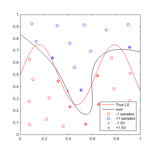
Train an SVM, then find and plot a "max-min" sample:

svm=CODES.fit.svm(x,y);
x_mm=CODES.sampling.mm(svm,[0 0],[1 1]);

[X,Y]=meshgrid(linspace(0,1,100));
Z=reshape(f([X(:) Y(:)]),100,100);

figure('Position',[200 200 500 500])
contour(X,Y,Z,[0 0],'r')
hold on
svm.isoplot('lb',[0 0],'ub',[1 1],'prev_leg',{'True LS'})
plot(x_mm(1),x_mm(2),'ms')
axis square

Comparison of Computational Time for: Parallel and Serial; Matlab and CODES MultiStart

Start a parallel pool:

gcp;

Compare compuational time of different scenarios to compute 10 "max-min":

CODES.common.disp_box('Using Matlab MultiStart')
tic;
svm=CODES.fit.svm(x,y);
CODES.sampling.mm(svm,[0 0],[1 1],'nb',10,'MultiStart','MATLAB');
disp(['Serial : ' CODES.common.time(toc)])
tic;
svm=CODES.fit.svm(x,y,'UseParallel',true);
CODES.sampling.mm(svm,[0 0],[1 1],'nb',10,'MultiStart','MATLAB');
disp(['Parallel : ' CODES.common.time(toc)])
CODES.common.disp_box('Using CODES MultiStart')
tic;
svm=CODES.fit.svm(x,y);
CODES.sampling.mm(svm,[0 0],[1 1],'nb',10,'MultiStart','CODES');
disp(['Serial : ' CODES.common.time(toc)])
tic;
svm=CODES.fit.svm(x,y,'UseParallel',true);
CODES.sampling.mm(svm,[0 0],[1 1],'nb',10,'MultiStart','CODES');
disp(['Parallel : ' CODES.common.time(toc)])

 
###########################
# Using Matlab MultiStart #
###########################
 
Serial : 17s
Parallel : 10s
 
##########################
# Using CODES MultiStart #
##########################
 
Serial : 15s
Parallel : 9s

Parallel update

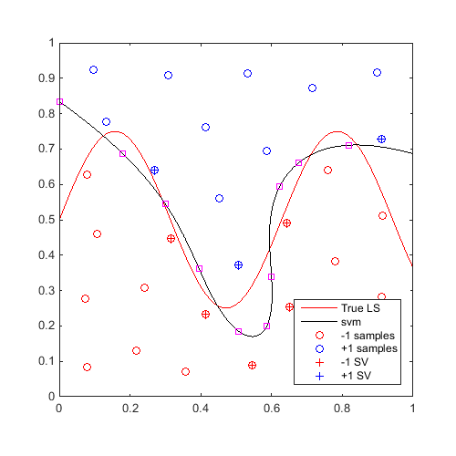
On the same example, find and plot 10 max-min samples:

f=@(x)x(:,2)-sin(10*x(:,1))/4-0.5;
x=CODES.sampling.cvt(30,2);
y=f(x);

svm=CODES.fit.svm(x,y,'UseParallel',true);
x_mm=CODES.sampling.mm(svm,[0 0],[1 1],'nb',10);

[X,Y]=meshgrid(linspace(0,1,100));
Z=reshape(f([X(:) Y(:)]),100,100);

figure('Position',[200 200 500 500])
contour(X,Y,Z,[0 0],'r')
hold on
svm.isoplot('lb',[0 0],'ub',[1 1],'prev_leg',{'True LS'})
plot(x_mm(:,1),x_mm(:,2),'ms')
axis square

Sequential refinement

On the same example, for 20 iterations, find a "max-min" sample and update the svm:

f=@(x)x(:,2)-sin(10*x(:,1))/4-0.5;
x=CODES.sampling.cvt(30,2);
y=f(x);

svm=CODES.fit.svm(x,y,'UseParallel',true);

[X,Y]=meshgrid(linspace(0,1,100));
Z=reshape(f([X(:) Y(:)]),100,100);

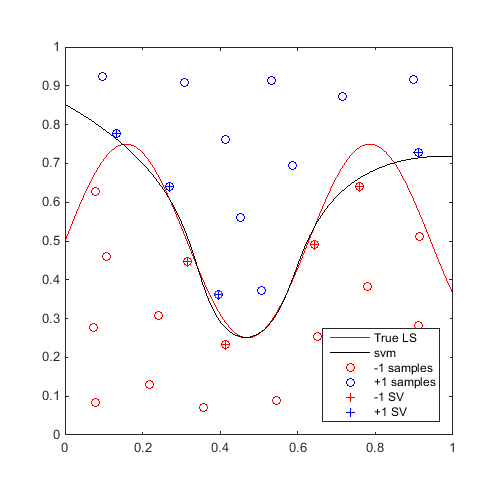
Plot first and last iteration:

x_mm=CODES.sampling.mm(svm,[0 0],[1 1]);
svm=svm.add(x_mm,f(x_mm));

figure('Position',[200 200 500 500])
contour(X,Y,Z,[0 0],'r')
hold on
svm.isoplot('lb',[0 0],'ub',[1 1],'prev_leg',{'True LS'})
plot(x_mm(:,1),x_mm(:,2),'ms')
axis square
axis square

for i=2:20
    x_mm=CODES.sampling.mm(svm,[0 0],[1 1]);
    svm=svm.add(x_mm,f(x_mm));
end

figure('Position',[200 200 500 500])
contour(X,Y,Z,[0 0],'r')
hold on
svm.isoplot('lb',[0 0],'ub',[1 1],'prev_leg',{'True LS'})
plot(x_mm(:,1),x_mm(:,2),'ms')
axis square
axis square

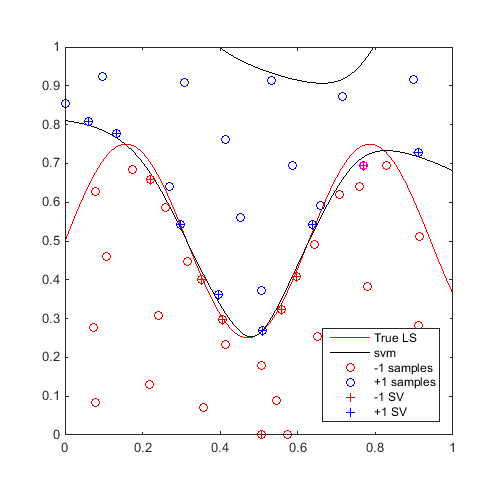
A video of this sequential update can be found here.

Copyright © 2015 Computational Optimal Design of Engineering Systems (CODES) Laboratory. University of Arizona.

Computational Optimal Design of Engineering Systems

Published with MATLAB® R2014b