CODES / sampling / mm

Find a "max-min" sample

Syntax
Description
Parameters
Example
Mini Tutorial
References
See also

Syntax

x_mm=CODES.sampling.mm(M,lb,ub) finds a "max-min" sample x_mm such that M.eval(x)=0 and lb < x < ub.
x_mm=CODES.sampling.mm(...,param,value) uses a list of parameters param and values value (c.f., parameter table).

Description

This function finds a "max-min" sample as introduced in Basudhar and Missoum (2010):

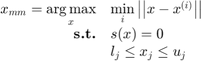
$\begin{array}{rl}x_{mm}=\mathop{\arg\max}\limits_{x}&\mathop{\min}\limits_{i}\left|\left|x-x^{(i)}\right|\right|\\\textbf{s.t.} & s(x)=0\\&l_j\leq x_j\leq u_j\end{array}$

where $x^{(.)}$ are the existing samples used to train $s$ , a meta-model (an SVM in Basudhar's work). The numerical implementation of this optimization problem follows the steps highlighted in Lacaze and Missoum (2014) regarding the use of the Chebychev distance (infinite norm). This problem being made differentiable, it is then solved using multi-start SQP.

Parameters

param value Description

'nb' positive integer, {1} Number of "max-min" samples requested ( 'nb' ≥ 2 is refered to as parallel, see Lin et al. (2012))

'intensity' positive integer, {30} Number of starting points for the multi-start SQP algorithm

'UseParallel' logical, {M.UseParallel} Should parallel setup be used

'MultiStart' {'CODES'}, 'MATLAB' Defines whether MATLAB or CODES multistart fmincon should be used.

'Display' {'off'}, 'iter', 'final' Defines the verbose level.

`param`	`value`	Description
'nb'	positive integer, {1}	Number of "max-min" samples requested ( 'nb' ≥ 2 is refered to as parallel, see Lin et al. (2012))
'intensity'	positive integer, {30}	Number of starting points for the multi-start SQP algorithm
'UseParallel'	logical, {`M.UseParallel`}	Should parallel setup be used
'MultiStart'	{'CODES'}, 'MATLAB'	Defines whether MATLAB or CODES multistart fmincon should be used.
'Display'	{'off'}, 'iter', 'final'	Defines the verbose level.

In addition, options from MultiStart can be used as well, when 'MultiStart' is set to 'MATLAB'.

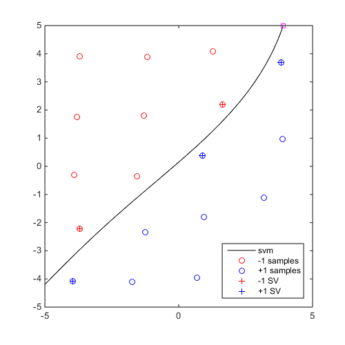
Example

Compute and plot a "max-min" sample

DOE=CODES.sampling.cvt(20,2,'lb',[-5 -5],'ub',[5 5]);
svm=CODES.fit.svm(DOE,DOE(:,1)-DOE(:,2));
x_mm=CODES.sampling.mm(svm,[-5 -5],[5 5]);
figure('Position',[200 200 500 500])
svm.isoplot('lb',[-5 -5],'ub',[5 5])
plot(x_mm(1),x_mm(2),'ms')

Mini Tutorial

A mini tutorial of the capabilities of the mm function.

References

Basudhar and Missoum (2010): Basudhar A., Missoum S., (2010) An improved adaptive sampling scheme for the construction of explicit boundaries. Structural and Multidisciplinary Optimization 42(4):517-529 - DOI
Lin et al. (2012): Lin S., Basudhar A., Missoum S., (2012) Parallel construction of explicit boundaries using support vector machines. Engineering Computations 30(1):132-148 - DOI
Lacaze and Missoum, (2014): Lacaze S., Missoum S., (2014) A generalized "max-min" sample for surrogate update. Structural and Multidisciplinary Optimization 49(4):683-687 - DOI