Examples / Reliability assessment / iform
This file is a complete demo of the capability of the iform function from the CODES toolbox.
Contents
Documentation
The documentation for the iform function can be found here. The examples used are taken from Youn et al. (2003).
Set rng
Set random number generator seed:
rng(0)
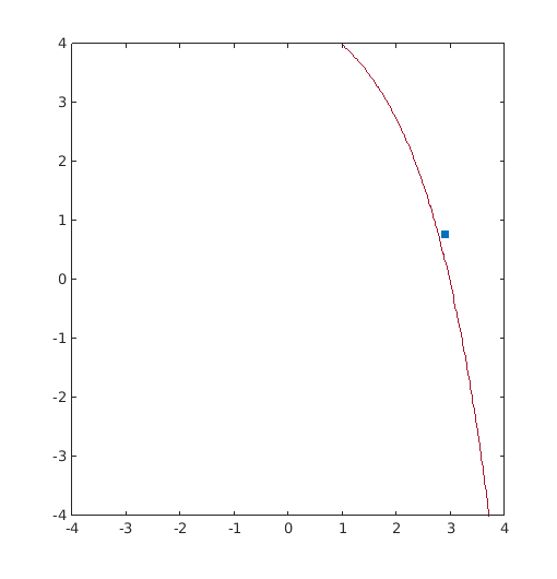
Example 1: Convex
Compute the MPTP on a simple 2D convex problem
g=@(x)-exp(x(:,1)-7)-x(:,2)+10;
T=@(x)(x-6)/0.8;
Tinv=@(u)u*0.8+6;

res_sqp=CODES.reliability.iform(g,2,3,'solver','sqp','Tinv',Tinv);
res_amv=CODES.reliability.iform(g,2,3,'solver','amv','Tinv',Tinv);
res_cmv=CODES.reliability.iform(g,2,3,'solver','cmv','Tinv',Tinv);
res_hmv=CODES.reliability.iform(g,2,3,'solver','hmv','Tinv',Tinv);

CODES.common.disp_matrix([res_sqp.LS_count res_sqp.MPTP res_sqp.PPM;...
                          res_amv.LS_count res_amv.MPTP res_amv.PPM;...
                          res_cmv.LS_count res_cmv.MPTP res_cmv.PPM;...
                          res_hmv.LS_count res_hmv.MPTP res_hmv.PPM],...
                         {'SQP','AMV','CMV','HMV'},...
                         {'# func. call','MPTP_1','MPTP_2','PPM'})
     # func. call   MPTP_1   MPTP_2        PPM
SQP            35  8.31845  6.62033  -0.357938
AMV            22  8.31827  6.62098  -0.357937
CMV            37  8.31765   6.6233  -0.357931
HMV            22  8.31827  6.62098  -0.357937
Provide plot
[X,Y]=meshgrid(linspace(-4,4,100));
Z=reshape(g(Tinv([X(:) Y(:)])),size(X));
figure('Position',[200 200 500 500])
Colors=get(gca,'ColorOrder');
contour(X,Y,Z,[0 0],'Color',Colors(end,:))
hold on
u_MPP=T(res_sqp.MPTP);
plot(u_MPP(1),u_MPP(2),'s',...
    'MarkerFaceColor',Colors(1,:),'MarkerEdgeColor',Colors(1,:))
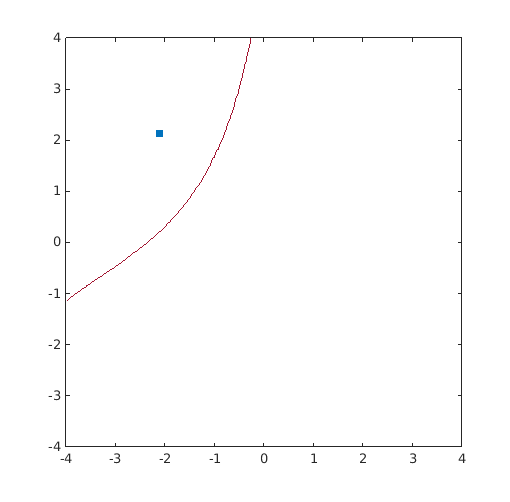
Example 2: Concave
Compute the MPTP on a simple 2D concave problem
g=@(x)(exp(0.8*x(:,1)-1.2)+exp(0.7*x(:,2)-0.6)-5)/10;
T=@(x)bsxfun(@rdivide,bsxfun(@minus,x,[4 5]),[0.8 0.8]);
Tinv=@(u)bsxfun(@plus,bsxfun(@times,u,[0.8 0.8]),[4 5]);

res_sqp=CODES.reliability.iform(g,2,3,'solver','sqp','Tinv',Tinv);
res_amv=CODES.reliability.iform(g,2,3,'solver','amv','Tinv',Tinv);
res_cmv=CODES.reliability.iform(g,2,3,'solver','cmv','Tinv',Tinv);
res_hmv=CODES.reliability.iform(g,2,3,'solver','hmv','Tinv',Tinv);

CODES.common.disp_matrix([res_sqp.LS_count res_sqp.MPTP res_sqp.PPM;...
                          res_amv.LS_count res_amv.MPTP res_amv.PPM;...
                          res_cmv.LS_count res_cmv.MPTP res_cmv.PPM;...
                          res_hmv.LS_count res_hmv.MPTP res_hmv.PPM],...
                         {'SQP','AMV','CMV','HMV'},...
                         {'# func. call','MPTP_1','MPTP_2','PPM'})
     # func. call   MPTP_1   MPTP_2       PPM
SQP            21   2.6807  2.99514  0.203815
AMV           301  1.98085  3.70268  0.379841
CMV            34  2.67694  2.99763   0.20382
HMV            34  2.67694  2.99763   0.20382
Provide plot
[X,Y]=meshgrid(linspace(-4,4,100));
Z=reshape(g(Tinv([X(:) Y(:)])),size(X));
figure('Position',[200 200 500 500])
Colors=get(gca,'ColorOrder');
contour(X,Y,Z,[0 0],'Color',Colors(end,:))
hold on
u_MPP=T(res_sqp.MPTP);
plot(u_MPP(1),u_MPP(2),'s',...
    'MarkerFaceColor',Colors(1,:),'MarkerEdgeColor',Colors(1,:))
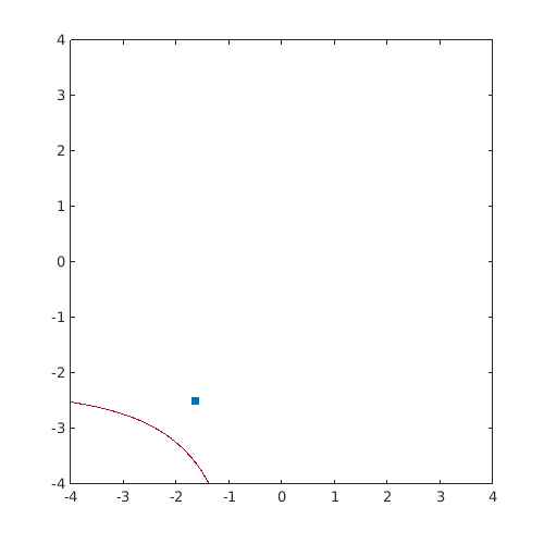
Example 3: Concave
Compute the MPTP on a simple 2D concave problem
g=@(x)0.3*x(:,1).^2.*x(:,2)-x(:,2)+0.8*x(:,1)+1;
T=@(x)bsxfun(@rdivide,bsxfun(@minus,x,[1.3 1]),[0.55 0.55]);
Tinv=@(u)bsxfun(@plus,bsxfun(@times,u,[0.55 0.55]),[1.3 1]);

res_sqp=CODES.reliability.iform(g,2,3,'solver','sqp','Tinv',Tinv);
res_amv=CODES.reliability.iform(g,2,3,'solver','amv','Tinv',Tinv);
res_cmv=CODES.reliability.iform(g,2,3,'solver','cmv','Tinv',Tinv);
res_hmv=CODES.reliability.iform(g,2,3,'solver','hmv','Tinv',Tinv);

CODES.common.disp_matrix([res_sqp.LS_count res_sqp.MPTP res_sqp.PPM;...
                          res_amv.LS_count res_amv.MPTP res_amv.PPM;...
                          res_cmv.LS_count res_cmv.MPTP res_cmv.PPM;...
                          res_hmv.LS_count res_hmv.MPTP res_hmv.PPM],...
                         {'SQP','AMV','CMV','HMV'},...
                         {'# func. call','MPTP_1','MPTP_2','PPM'})
     # func. call     MPTP_1   MPTP_2       PPM
SQP            26   0.140039  2.17345  -1.04864
AMV            73   0.153993  2.18708  -1.04833
CMV            16  0.0794953  2.11035  -1.04275
HMV            16  0.0794953  2.11035  -1.04275
Provide plot
[X,Y]=meshgrid(linspace(-4,4,100));
Z=reshape(g(Tinv([X(:) Y(:)])),size(X));
figure('Position',[200 200 500 500])
Colors=get(gca,'ColorOrder');
contour(X,Y,Z,[0 0],'Color',Colors(end,:))
hold on
u_MPP=T(res_sqp.MPTP);
plot(u_MPP(1),u_MPP(2),'s',...
    'MarkerFaceColor',Colors(1,:),'MarkerEdgeColor',Colors(1,:))
Sensitivities
Here is ans example on how to compute sensitivities of the probabilistic performance measure. See iform help for details on the options.
g=@(x,z)CODES.test.lin([x repmat(z,size(x,1),1)]);
T=@(x,mu)norminv(expcdf(x,mu));
Tinv=@(u,mu)expinv(normcdf(u),mu);

z=0;
mu=0.5;
delta=1e-3;

res_iform=CODES.reliability.iform(@(x)g(x,z),2,2,...
    'Tinv',@(x)Tinv(x,mu),'eps',1e-5,'gz',g,'z',z,...
    'Tinvtheta',Tinv,'T',T,'theta',mu);
res_iform_theta=CODES.reliability.iform(@(x)g(x,z),2,2,...
    'Tinv',@(x)Tinv(x,mu+delta),'eps',1e-5);
res_iform_z=CODES.reliability.iform(@(x)g(x,z+delta),2,2,...
    'Tinv',@(x)Tinv(x,mu),'eps',1e-5);

dGdmu=(res_iform_theta.PPM-res_iform.PPM)/delta;
dGdz=(res_iform_z.PPM-res_iform.PPM)/delta;

CODES.common.disp_matrix([dGdz res_iform.dPPMdz;dGdmu res_iform.dPPMdtheta],...
    {'dPPM/dz','dPPM/dtheta'},...
    {'FD','Analytical'})
                   FD  Analytical
    dPPM/dz  -0.57735    -0.57735
dPPM/dtheta  -2.93612    -2.93612
References
- Youn et al. (2003): Youn, B. D., Choi, K. K., & Park, Y. H. (2003). Hybrid Analysis Method for Reliability-Based Design Optimization. Journal of Mechanical Design, 125(2), 221. DOI
Copyright © 2015 Computational Optimal Design of Engineering Systems (CODES) Laboratory. University of Arizona.
|
|
Computational Optimal Design of Engineering Systems |

|