Examples / Reliability assessment / subset

This file is a complete demo of the capability of the subset function from the CODES toolbox.

Contents

Documentation

The documentation for the subset function can be found here.

Set rng

Set random number generator seed:

rng(0)

Complex example

Compare FORM, SORM, Subset and MC

g=@(x)-(x(:,1)+x(:,2)).^2+20;
res_form=CODES.reliability.form(g,2,'solver','hl-rf');
res_sorm=CODES.reliability.sorm(g,2,'res_form',res_form);
res_subset=CODES.reliability.subset(g,2,'vectorial',true);
res_mc=CODES.reliability.mc(g,2,'vectorial',true);

CODES.common.disp_matrix(...
    [res_form.beta res_sorm.beta res_subset.beta res_mc.beta;...
    res_form.Pf res_sorm.Pf res_subset.Pf res_mc.Pf;...
    res_form.LS_count res_sorm.LS_count res_subset.LS_count res_mc.LS_count],...
    {'Beta','Pf','# funct. calls'},{'FORM','SORM','SubSim','MC'})

                       FORM        SORM      SubSim        MC
          Beta      3.16228     3.05994     2.95188    2.9492
            Pf  0.000782701  0.00110692  0.00157922  0.001593
# funct. calls           73           9      268024     1e+06

Compute and compare sample coefficient of variation of SubSim and MC

for i=1:200
    res_subset(i)=CODES.reliability.subset(g,2,'vectorial',true);
    res_mc(i)=CODES.reliability.mc(g,2,'vectorial',true);
end

CODES.common.disp_matrix(...
    [mean(cell2mat({res_subset.LS_count})) mean(cell2mat({res_mc.LS_count}));...
    mean(cell2mat({res_subset.beta})) mean(cell2mat({res_mc.beta}));...
    mean(cell2mat({res_subset.Pf})) mean(cell2mat({res_mc.Pf}));...
    100*std(cell2mat({res_subset.beta}))/mean(cell2mat({res_subset.beta})) 100*std(cell2mat({res_mc.beta}))/mean(cell2mat({res_mc.beta}));...
    100*std(cell2mat({res_subset.Pf}))/mean(cell2mat({res_subset.Pf})) 100*std(cell2mat({res_mc.Pf}))/mean(cell2mat({res_mc.Pf}))],...
    {'# funct. calls','E[Beta]','E[Pf]','cv Beta','cv Pf'},{'SubSim','MC'})

                    SubSim         MC
# funct. calls      268088      1e+06
       E[Beta]     2.95462    2.95534
         E[Pf]  0.00156577  0.0015622
       cv Beta    0.280376   0.295351
         cv Pf     2.67647    2.82895

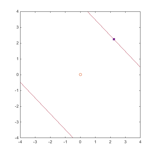
Plot the limit state

figure('Position',[200 200 500 500])
[X,Y]=meshgrid(linspace(-4,4,100));
Z=reshape(g([X(:) Y(:)]),size(X));
Colors=get(gca,'ColorOrder');
contour(X,Y,Z,[0 0],'Color',Colors(end,:))
hold on
plot(res_form.MPP(1),res_form.MPP(2),'s','MarkerFaceColor',Colors(4,:),'MarkerEdgeColor',Colors(4,:))
plot(0,0,'o')

Change the target distribution

In this example, consider same limit state function but we modify the marginal PDFs. For example, if the two random variables follow gaussian distribution with respective means 1 and 0 and respective standard deviation 1 and 0.5:

pdfs_target=@(x)normpdf(x,repmat([1 0],size(x,1),1),repmat([1 0.5],size(x,1),1));
sampler=@(N)normrnd(repmat([1 0],N,1),repmat([1 0.5],N,1));
res_subsim=CODES.reliability.subset(g,2,'vectorial',true,'PDFs_target',pdfs_target,'sampler',sampler);
disp(res_subsim);

          Pf: 9.2893e-04
        beta: 3.1121
       steps: 4
    LS_count: 341035

Compute sensitivities dPfdtheta

Here are two examples on how to compute sensitivities of the estimated probability of failure. See subset help for details on the options.

Using a simple standard gaussian space and a linear limit state:

d=3;
g=@(x)-x(:,2)-x(:,1)+d;
beta=@(mus)(d-sum(mus))/sqrt(2);
dbetadtheta=-1/sqrt(2)*ones(1,2);
dPdfdtheta=@(mus)-dbetadtheta*normpdf(-beta(mus));

lnPDF=@(x,mus)sum(log(normpdf(x,mus,[1 1])),2);
dlnPDF=@(x,mus)bsxfun(@minus,x,repmat(mus,size(x,1),1));

tic;
res_subset=CODES.reliability.subset(g,2,'vectorial',true,'lnPDF',lnPDF,'theta',[0 0]);
time_ln=toc;
tic;
res_subset1=CODES.reliability.subset(g,2,'vectorial',true,'dlnPDF',@(x)dlnPDF(x,[0 0]));
time_dln=toc;

CODES.common.disp_matrix([res_subset.dPfdtheta res_subset.dbetadtheta time_ln;...
    res_subset1.dPfdtheta res_subset1.dbetadtheta time_dln;
    dPdfdtheta([0 0]) dbetadtheta 0],{'ln','dln','ref'},...
    {'dPfdtheta1','dPfdtheta2','dbetadtheta1','dbetadtheta2','time'});

     dPfdtheta1  dPfdtheta2  dbetadtheta1  dbetadtheta2       time
 ln   0.0296094   0.0298026      -0.70314     -0.707728    22.1964
dln   0.0299514   0.0297982     -0.709238     -0.705612  0.0898568
ref   0.0297326   0.0297326     -0.707107     -0.707107          0

Compute sensitivities dPfdz

Using a simple standard gaussian space and a linear limit state:

d=4;
z=[1 2];
gg=@(x)deal(-sum(z)-x+d,-ones(size(x,1),2));
g=@(x)-z-x+d;
Pf=@(z)1-normcdf(d-sum(z));
beta=@(z)-norminv(Pf(z));
dPfdz=@(z)normpdf(d-sum(z));
dbetadz=@(z)-dPfdz(z)/normpdf(-beta(z));

res_subset=CODES.reliability.subset(gg,1,'vectorial',true,'nz',2,'frac',0.5,'dirac','gauss');

CODES.common.disp_matrix([res_subset.dPfdz res_subset.dbetadz;...
    dPfdz(z) dPfdz(z) dbetadz(z) dbetadz(z)],{'est','ref'},...
    {'dPfdz1','dPfdz2','dbetadz1','dbetadz2'});

       dPfdz1    dPfdz2   dbetadz1   dbetadz2
est  0.237711  0.237711  -0.991311  -0.991311
ref  0.241971  0.241971         -1         -1

Copyright © 2015 Computational Optimal Design of Engineering Systems (CODES) Laboratory. University of Arizona.

Computational Optimal Design of Engineering Systems

Published with MATLAB® R2014b